Multivariate probability generating functions

While one can go a long way with univariate generating functions, it is limited to characterize a single random variable—or the sum of multiple independent random variables—, but to characterize \(m\) random variables \((n_1, n_2, \dots, n_m)\) that are not necessarily independent, we need to consider multivariate probability generating functions of the form

\[ \begin{align} G(x_1,x_2,\dots,x_m) = \sum_{n_1 = 0}^\infty \cdots \sum_{n_m = 0}^\infty p_{n_1,n_2,\dots,n_m} x_1^{n_1}x_2^{n_2} \cdots x_m^{n_m} \;, \end{align} \]

where \(p_{n_1,n_2,\dots,n_m}\) is the joint probability distribution.

Fortunately, all the properties we discussed previously and the numerical inversion can still be applied.

Playing craps the hard way

In a regular game of scraps, the goal is to predict the outcome of a roll of two six-sided dice. But we care about each die and not just the sum of their results! For instance, rolling a 4, 6, 8, or 10 as both dice giving the same number is called a “hard number,” because it’s rolled the “hard way”. Our previous approach to rolling two dice would simply sum their results and generate the outcome with \(g_6(x)^2\) such that a 4 and a 2 is the same as two 3s! How can we calculate the probability of rolling a 6 the hard way? We keep track of each outcome independently!

\[ h_6(x_1,x_2,x_3,x_4,x_5,x_6) = \sum_{n=1}^6 \frac{x_n}{6} \]

So what is the probability of a 6 the hard way? It is generated by the following PGF and associated with its \(x_3^2\) coefficient since it involves 2 rolls of 3.

\[ h_6(x_1,x_2,x_3,x_4,x_5,x_6)^2 \]

Throwing dice of different colors

Let’s assume we throw three fair dice. Two of the three are blue and one is red (call this one a bonus). We calculate two sums (\(n_1\) and \(n_2\)) by adding the number on top of the red die with the two numbers on top of the blue dice independently. So, if the red die reads 2 while the blue dice read 4 and 5, we get two numbers by adding our bonus to the two blue dice: \(n_1=4+2=6\) and \(n_2=5+2=7\). What is the PGF for \(p_{n_1,n_2}\)? It is

\[ \begin{align} G(x_1,x_2) = g_6(x_1) g_6(x_2)g_6(x_1x_2) \;. \end{align} \]

Indeed, if \(k_1\) and \(k_2\) are the number on top of the blue dice, and \(k_3\) is the result on top of the red die,

\[\begin{split} \begin{align} G(x_1,x_2) &= \sum_{n_1=0}^{12} \sum_{n_2=0}^{12} p_{n_1,n_2} x_1^{n_1} x_2^{n_2} \;, \\ &= \sum_{k_1=0}^{6} \sum_{k_2=0}^{6} \sum_{k_3=0}^{6} p_{k_1} p_{k_2} p_{k_3} x_1^{k_1 + k_3} x_2^{k_2 + k_3} \;, \\ &= \sum_{k_1=0}^{6} p_{k_1} x^{k_1} \sum_{k_2=0}^{6} p_{k_2} x^{k_2} \sum_{k_3=0}^{6} p_{k_3} (x_1x_2)^{k_3} \;, \\ &= g_6(x_1) g_6(x_2)g_6(x_1x_2) \;, \end{align} \end{split}\]

So, despite the fact that \(n_1\) and \(n_2\) are not independent, we can still use the independence of the underlying dice throw (\(k_1\),\(k_2\), and \(k_3\)) to construct the joint PGF by the multiplication of the PGFs representing the independent random variables.

Numerical inversion of multivariate PGFs

Similarly to the univariate case, the joint distribution \(p_{n_1,n_2}\) is recovered from the multivariate PGF \(G(x_1,x_2)\) using a discrete Fourier transform

\[ \begin{align} p_{n_1,n_2} = \frac{1}{N_1 N_2 r_1^{n_1} r_2^{n_2} } \sum_{m_1 = 0}^{N_1-1} \sum_{m_2 = 0}^{N_2-1} G\left(r_1 e^{2 \pi i m_1 /N_1}, r_2 e^{2 \pi i m_2 /N_2} \right) e^{2 \pi i n_1 m_1 /N_1}e^{2 \pi in_2 m_2 /N_2 } \;. \end{align} \]

Again, \(r_1\) and \(r_2\) are the radii of the contour of integration in both dimensions and should be chosen wisely to limit the effect of aliasing if \(N_1\) and \(N_2\) are too small.

import numpy as np
import matplotlib.pyplot as plt
plt.style.use(['seaborn-talk'])

g = lambda x: np.sum([x**n/6 for n in range(1,7)])
G = lambda x1,x2: g(x1)*g(x2)*g(x1*x2)
G = np.vectorize(G)
N1 = 13
N2 = 13
n1 = np.arange(N1)
n2 = np.arange(N2)
c1 = np.exp(2*np.pi*1j*n1/N1)
c2 = np.exp(2*np.pi*1j*n2/N2)
C1, C2 = np.meshgrid(c1, c2) #get 2d array versions
pn1n2 = abs(np.fft.fft2(G(C1,C2))/(N1*N2))
plt.imshow(pn1n2, origin='lower')
plt.colorbar(label='Probability')
plt.ylabel(r'$n_1$')
plt.xlabel(r'$n_2$')
plt.show()

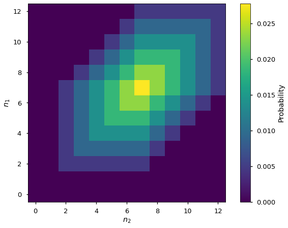
Try playing with both the dimensions (\(N_1,N_2\)) and the radii (\(r_1,r_2\)) to see the impact.