Exercises part II: branching process#
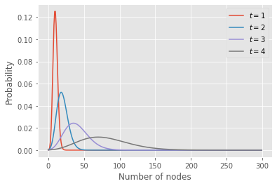
The code below extract the probability distribution for the number of nodes at a few time points for a branching process with a Poisson offspring distribution.
import numpy as np
import matplotlib.pyplot as plt
plt.style.use(['ggplot'])

R = 2.
Q = lambda x: np.exp(R*(x-1))
G0 = lambda x: x**5
N = 300
n = np.arange(N)
c = np.exp(2*np.pi*1j*n/N)

tset = {1,2,3,4}
x = c.copy()
for t in range(max(tset)+1):
    if t in tset:
        pn = abs(np.fft.fft(G0(x))/N)
        plt.plot(n,pn, label=fr"$t = {t}$")
    x = Q(x)
plt.legend()
plt.ylabel('Probability')
plt.xlabel('Number of nodes')
plt.show()
Modeling overdispersion#
Change the offspring distribution to a negative binomial, using the PGF
Use different values of \(\kappa > 0\) and see what happens. Take a very large value of \(\kappa\) and compare with the Poisson case.
Tip
Remember to adapt the support to avoid aliasing effects.
Probability of extinction#
Set \(\kappa = 0.1\) and now extend the time to a large value (e.g., \(t = 10\) should be enough). You should observe that \(p_0\) (the probability of extinction) converge to a certain value.
Change the initial condition \(G_0(x)\) and see how this affects \(p_0\) for large \(t\).
Now vary \(R\). Can you find a critical value \(R_\mathrm{c}\) such that \(p_0 = 1\) (for large \(t\)) for all \(R < R_\mathrm{c}\)? Does this value depend on \(G_0(x)\) or \(\kappa\)?