Exercises part III: statistical inference

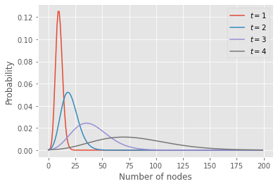
The code below extract the probability distribution for the number of nodes at a few time points for a branching process with a Poisson offspring distribution.

import numpy as np
import matplotlib.pyplot as plt
plt.style.use(['ggplot'])

R = 2.
Q = lambda x: np.exp(R*(x-1))
G0 = lambda x: x**5
N = 200
n = np.arange(N)
c = np.exp(2*np.pi*1j*n/N)

tset = {1,2,3,4}
x = c.copy()
for t in range(max(tset)+1):
    if t in tset:
        pn = abs(np.fft.fft(G0(x))/N)
        plt.plot(n,pn, label=fr"$t = {t}$")
    x = Q(x)
plt.legend()
plt.ylabel('Probability')
plt.xlabel('Number of nodes')
plt.show()

Tip

Remember to adapt the support to avoid aliasing effects.

Posterior distribution on the reproduction number

Let us assume that we have an emerging outbreak. To simplify the situation, let us assume that the generation time is always a week, and infectious individuals generate a number of secondary case according to a Poisson distribution with PGF of the form

\[ \begin{align} Q(x) = e^{R(x-1)}\;. \end{align} \]

We can model this situation using a branching process, and we want to infer \(R\), the reproduction number.

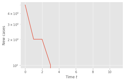
Run the code below to get a time series—this will represent the data available.

from secret_code import *
T = 12 #length of the time series
t = np.arange(T)
n = poisson_branching_process(T)

plt.semilogy(t,n)
plt.xlabel(r"Time $t$")
plt.ylabel(r"New cases")
plt.show()

Reusing the code above for the PGF, estimate the posterior distribution on \(R\).

Tip

As a first step, use only the first and last data points, \(n_0 = 1\) and \(n_T\). You have that \(G_0(x) = x^{n_0}\), and you can calculate \(G_T(x)\) (and the associated probability distribution) from the recursion implemented in the code above.

The posterior distribution is \(P(R|n_0,n_T) \propto P(n_T| n_0, R) P(n_0,R)\). We could choose different prior distribution, but right now let us assume that \(P(n_0,R)\) is simply some constant \(C\).

Since the likelihood \(P(n_T| n_0, R)\) is generated by \(G_T(x)\), we can evaluate the posterior distribution for a few values of \(R\) on an interval and plot the resulting curve.

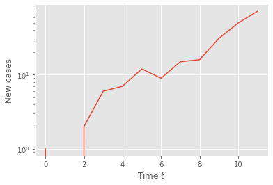
To make it a bit more realistic, apply your code to the following time series, where only a certain fraction of the cases are detected.

from secret_code import *
T = 12 #length of the time series
t = np.arange(T)
n = poisson_branching_process_with_noise(T)

plt.semilogy(t,n)
plt.xlabel(r"Time $t$")
plt.ylabel(r"New cases")
plt.show()

Try using more data points and breaking down the likelihood in a product (see below). Is the inference better?

\[ \begin{align} \prod_{j=1}^{T/\tau} P\left(n_{j\tau}|n_{(j-1)\tau}, R\right) \;. \end{align} \]

Note

In the limit \(\tau = 1\), one could argue (successfully) that PGFs are not necessary here. Indeed, \(P(n_{t}|n_{t-1},R)\) is a Poisson distribution by the additive property of Poisson random variables. While this is true in this very simple exercise, realistic situations will lead to a much more complex likelihood which either require PGFs, or an approximation scheme making use of simulation like approximate Bayesian computation (ABC).